
Tutorial P2P - Loading and Understanding the Complete Basic Model
TL;DR
Goal: Switch from the manually built exercise model to the full Simple P2P base model.
Prerequisites: The basic table, approval and 1:N logic from the previous articles is understood.
Result:Config 1 – Basisis loaded and forms the starting point for all subsequent business use cases.
Why are we switching to a prepared config now?
In the previous steps we deliberately built only a portion of the P2P model ourselves.
This allowed us to follow the most important fundamentals:
- tables and primary keys,
- foreign keys,
- primary and additional timestamps,
- the causal chain
Causal Chain, - branches and joins,
- as well as the 1:N relationship between
bestellungandbestellposition.
For the following use cases, however, we now need a more extensive data set.
Maverick buying, for example, requires information about the anforderer. Supplier performance requires a lieferant. Loss of cash discount requires invoice, approval and payment information.
Instead of creating all these tables and attributes individually by hand, we now switch to a defined initial state.
1. Loading Config 1 – Basis
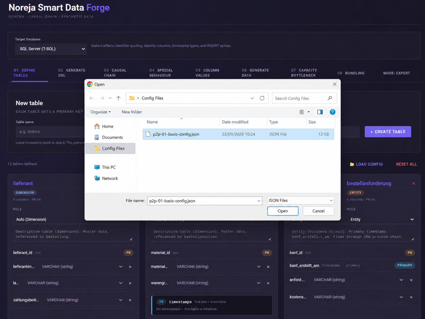
Use: Load config and choose: p2p-01-basis-config.json
Important: Load config does not add to the existing state.
The loaded config completely replaces the current working state. Tables, slots, column values, run settings and all other saved settings are taken from the config.
The previously hand-built state is thus deliberately left behind.
What does the base config contain?
After loading, twelve tables are available:
Reference and master data
lieferant, material, vertrag
These objects represent business information that is referenced by the actual process objects.
They are not placed as their own process steps in the causal chain Causal Chain, but are generated as master data Reference data.
Process objects
bestellanforderung, freigabe_a, freigabe_b, bestellung, bestellposition, wareneingang, rechnung, rechnung_freigabe, zahlung
This means we now have a complete simplified P2P process from the requisition through to payment.
The process chain of the base config
Under 03 Causal Chain you will now find the following business base structure:
bestellanforderung
→ Approval logic: Direct XOR Dual (approval(s))
→ bestellung
→ bestellposition
→ wareneingang
→ rechnung
→ rechnung_freigabe
→ zahlung
The approval structure already introduced remains in place.
The relationship:
bestellung → bestellposition
is also still modeled with a cardinality of 1 to 3 order line items and skew low.
Why are delivery and goods inspection missing?
The base model is deliberately not yet the full Expert model.
Objects such as:
lieferung
warenannahme
bereitstellung
wareneingang_pruefung
are only added later.
They are needed when we examine different procurement paths as well as capacity bottlenecks and delay propagation.
For the first business use cases, this additional structure would make getting started unnecessarily complex.
That is why we initially work with a simplified chain:
bestellposition → wareneingang → rechnung
Only in Expert Mode does this become a more differentiated process.
Still a clean world
A particularly important point about the base config:
No business process deviations are configured yet.
Under 04 Special Behaviour there are initially no rules.
So there is not yet any:
- maverick buying,
- rework,
- wrong order,
- or deliberately generated process abort.
The Conditional Rules, with which we later model, for example, supplier performance or working-capital effects, are also still deliberately empty.
Column Values are already prepared
Although there are no process deviations yet, the base config already contains value configurations for the business attributes.
This means we do not have to reconfigure supplier names, requesters, product groups, amounts or other base values anew for every article.
The separation is important:
Column Values determine which values occur in the data.
Special Behaviour and Conditional Rules determine how certain cases or values affect the process.
A supplier named Globex SE is thus initially simply just a supplier.
It only becomes our example of poor supplier performance once we later add a rule that causes longer process times for this supplier.
Reference Data
Under Causal Chain → Reference data you will find the tables that are not themselves used as a process step.
In our base, the following in particular:
lieferant , material, vertrag
are such reference objects.
The config generates a defined number of records from these. Process objects can then refer to this master data via their foreign keys.
This later enables analyses such as:
- cycle time by supplier,
- process behavior by material,
- orders with or without a contract reference.
The master data therefore does not itself become process activities, but provides important analysis dimensions.
Checking the run settings
The tutorial config still uses:
| Setting | Value |
|---|---|
| Number of cases | 500 |
| Start date | 2025-01-01 |
| Span (days) | 90 |
| Seed | 42 |
| Target Database | SQL Server |
| Mode | Simple |
The seed stays the same throughout the training.
This lets us compare the effects of our changes more easily: differences between two runs do not arise merely from a completely new random population, but primarily from the rules we add.
Our starting point for the next articles
From now on, all Simple articles build on this state.
So we do not reload the base config before every article.
Instead, we extend the same model one step at a time:
Base
→ Maverick buying
→ poor supplier performance
→ order change / rework
→ wrong order
→ process abort / open processes
→ working capital and loss of cash discount
After the final step, our self-built state corresponds, in business terms, to:
Config 2 – Simple
This second config serves as a reference in case an intermediate state is lost or you want to check your own result.
Save config can be used at any time in between, but is not required for each individual article.
What we deliberately do not do yet
We do not yet configure any:
Capacity Bottleneck rules,
- backlogs,
- delay propagation,
- bundling runs,
- physical / software process paths.
We cover these functions together in the later Expert part.
Next step: Maverick Buying
Our first business scenario is:
Are orders carried out without the approval that is actually intended?
For this we use the already existing approval structure and add a Special Behaviour for the first time.
Certain requesters will deliberately bypass the approval path that is actually intended.
In doing so, we also get to know an important distinction:
A regular DIRECT path is an intended process variant.
Maverick buying, by contrast, is a deliberately generated deviation from the expected approval behavior.
In the next article we configure exactly this difference with Team bypass.